
Level-1A download as bunzip2 files, which extract to an hdf4 file
Level-2 files are netCDF / hdf5
Estimated time to complete: 4-8 hours
This should be completed before the start of the lab.
Install SeaDAS version 8.3 and up.
Once up and running, install OCSSW data processing components for MODIS-Aqua (instructions below the SeaDAS download instructions on the SeaDAS website). Take particular note of the system and software requirements for installation. One issue that has recurred is the absence of a requests library in python. One example way to resolve this is running the following from a terminal window:
/usr/bin/python3 -m pip install --user requests
You will also need to set up an Earthdata login . Your login credentials then need to be stored in a file in your home directory. In your home directory, create a file called .netrc (note the leading period) using the terminal:
echo "machine urs.earthdata.nasa.gov login USERNAME password  PASSWD" > ~/.netrc ; > ~/.urs_cookies

chmod  0600 ~/.netrc
where USERNAME and PASSWD are your Earthdata Login credentials.
All SeaDAS data processing functions are available through a GUI and a command line executable. Using the latter requires setting up the proper command line environment.
Open a terminal window. Locate your OCSSW software installation (path).
By default, this should be a subdirectory within your SeaDAS installation. For example: /Applications/seadas/occsw .
Define an environmental variable called OCSSWROOT that points to your OCSSW software installation. The language for doing so depends on your shell. On Macs, the default is bash:
export OCSSWROOT=/[Path to SeaDAS OCSSW folder]
e.g.
export OCSSWROOT=/Applications/seadas/ocssw
Confirm the installation via the command:
printenv OCSSWROOT
This should print the [path to SeaDAS] that you entered to your terminal screen.
Finish setting up the command line environment by sourcing the data processing environmental variable file. This file defines the locations of all files required by OCSSW. In bash:
source $OCSSWROOT/OCSSW_bash.env
Confirm the environment has been set via the command:
which l2gen
This should print the full path to the file l2gen to your terminal screen (e.g., /Applications/seadas/ocssw/bin/l2gen ).
If you experienced an OCSSW install error in Section 0, you may also need to run the following from a terminal window to complete installation of required satellite data files:
update_luts [sensor name]
e.g.
update_luts modisa

update_luts viirsj1
See the SeaDAS web site for identification of recognizable instrument names.
Next, let's locate, download, and identify the file type of Level-1A and -2 satellite data. We will use these files over the course of this lab.
Acquire the following MODIS-Aqua files from the OceanColorWeb Level-1/2 browser . They encompass 3 successive days in the Gulf of Maine - 29 Sep 2018 to 1 Oct 2018:
The above provides everything you need to know to find these files.
Level-1A download as bunzip2 files, which extract to an hdf4 file
Level-2 files are netCDF / hdf5
It's time to open SeaDAS.
Full granules can be large. Images with lots of water can take a significant amount of time to process from Level-1 to -2. Let's extract our region of interest, the Gulf of Maine, defined here as:
40° to 46° N, and
-75° to -60° W
You will need to open the full files in SeaDAS first; either by going into File > Open Product or by dragging and dropping the files into the SeaDAS file manager.
Go to SeaDAS-Toolbox > SeaDAS Processors > extractors
Do the Level-2 files first, using the above latitude and longitude
boundaries to define the extract.
Do not run the extractor yet
. You'll notice that the start and end pixel and line number fields get
populated after you've added the latitude and longitude boundaries. Write
these down. You will need them to run the Level-1A extracts.

| File | spixl | epixl | sline | eline |
|---|---|---|---|---|
| A2018272172500.L1A_LAC | 270 | 1278 | 1 | 774 |
| A2018273180500.L1A_LAC | 1 | 675 | 1109 | 1890 |
| A2018274171000.L1A_LAC | 450 | 1345 | 976 | 1924 |
Another way of extracting with SeaDAS is to make a subset using Raster > Subset and to enter the boundaries, like you would with the extractor. That also allows you to choose the bands that you want to keep in your subset. The created file then needs to be saved.
Level-2 files have been geolocated and, thus, include latitude and longitude information.
Level-1A files have not been geolocated and, thus, latitudes and longitudes are not yet assigned to each pixel.
Once you've created the six extracts, you can close the full files for the remainder of this lab.
MODIS-Aqua Level-1A files need to be geolocated before Level-2 files can be generated. Note, this is not true for all ocean color satellites - SeaWiFS, for example, does not require this step. This doesn't mean that SeaWiFS files aren't geolocated, only that this process is consolidated elsewhere in the SeaWiFS data processing architecture.
Use the OCSSW MODIS GEO processor to geolocate 1 or 2 of the 3 Level-1A extracts using default options.
All SeaDAS data processing GUIs list the name of their corresponding command line executable on the top bar of the GUI window.
modis_GEO.py
$OCSSWROOT/scripts/
Python
Run the MODIS GEO script from your terminal window without any inputs:
modis_GEO
Help and usage information will scroll in your terminal window. All SeaDAS command line executables do this when you run the command without input variables. If you've set up the terminal environment correctly, you do not need to provide the full paths to the executables to run them.
Use the command line to geolocate the remaining 1 or 2 L1A extracts .
First, cd into your folder so that your files save in the right place:
cd [path to your folder]
e.g.
cd /accounts/cpoulin/SeaDAS
Then create de GEO file:
modis_GEO [L1Afile (path+L1A filename)]
e.g.
modis_GEO /Applications/seadas/data/A2018272172500.L1A_LAC
MODIS-Aqua Level-1A files need to be processed to Level-1B before Level-2 files can be generated. Again, not all ocean color satellites require this independent processing step.
Use the OCSSW MODIS L1B processor to generate Level-1B files. Consider using both the GUI and the command line. Do not provide any inputs other than the Level-1A and GEO file names:
modis_L1B [L1Afile] [GEOFILE]
3
LAC file has the 1 km data products
HKM files have the 500-m bands (469, 555, 1240, 1640, 2130 nm)
QKM files have the 250-m bands (645, 859 nm)
We will not be using the HKM or QKM files the remainder of this lab.
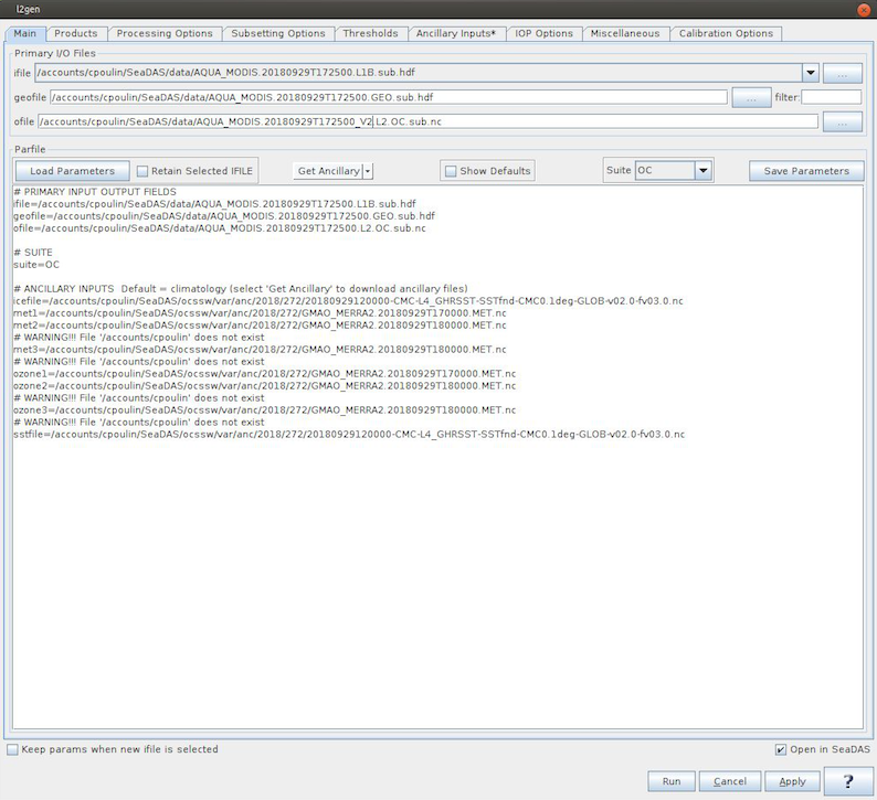
The "l2gen" executable in SeaDAS provides Level-2 processing capabilities for all ocean color instruments under the auspices of the GSFC Ocean Biology Processing Group. When you run l2gen without any inputs (other than the input file names and ancillary data file names), you will exactly recreate the Level-2 files distributed on the OceanColorWeb.
Open the OCSSW l2gen processor GUI.
Select the extracted AQUA_MODIS.20180929T172500* L1B as ifile. If you have a Level-1B file highlighted in the File Manager window, the geofile and ofile fields will self-populate.
Rename the ofile - otherwise, you may overwrite the Level-2 extract you previously created.
Acquire the ancillary data associated with this data file (hint: there is a
GUI button). Run l2gen.
Open the Level-2 extract you created previously and the Level-2 file that you just produced.
There may be an offset in the geographic boundaries of the imagery, but the geophysical data and its spatial patterns should be identical.
Repeat for the other 2 Level-1B extracts. Continue until you are convinced that the Level-2 files you generate are identical to the Level-2 extracts you created previously. This is also a good way to verify that you ran the extractor properly.
Without exaggeration, l2gen can produce hundreds of geophysical data products and be configured in thousands of different combinations.
Open the l2gen GUI and explore the tabs.
Note several highlights: The "Processing Options" and "Ancillary Inputs" tabs, the "IOP Options" tab, and the band-ratio chlorophyll algorithms can be tuned in the "Miscellaneous" tab.
To run l2gen from the command line:
l2gen par=[parameter file]
where the parameter file includes a list of keyword=value pairs (one per line).
Note that you can also run l2gen from the command lines as:
l2gen header1=keyword1 header2=keyword2 header3=keyword3
… (and so on)
-For a complete GUI-based list of these keyword=value pairs, select the "Show Defaults" button under the "Main" tab. This will list all of the keyword=value pairs with the default values used in standard processing. For a complete terminal-based list, run
l2gen
from the command line without any inputs.
- l2gen does not require providing a keyword=value pair to use a default configuration, which is why they are commented out in this "Show Defaults" display (the "#" at the beginning of the line tells l2gen to ignore that line). To use an alternate l2gen setting in the GUI, you can either make the change in one of the tabs or you can edit the keyword values within the "Main" tab display by removing the "#" and changing the value.
- A parameter file only needs to include those values that diverge from their defaults. This is why we didn't need to change anything in the previous exercise to exactly replicate the standard Level-2 files distributed online. The "Main Tab" always shows those keyword=value pairs that diverge from the default configuration.
- You can download a parameter file developed within the GUI using the "Save Parameters" button. Likewise, you can also load one using "Load Parameters".
Let's explore how a geophysical data product changes when we diverge from the default configuration of l2gen. Use the AQUA_MODIS.20180929T172500* L1B and GEO files for this exercise.
We will rerun l2gen 3 times. Make sure to rename the ofile for each instance or you will overwrite the Level-2 file(s) that you previously generated.
9.1 Generate a Level-2 file using climatological ancillary data. This is exactly the same as the exercise in Section 7, but without hitting the "Get Ancillary" button.
Chl differences from change in ancillary data:
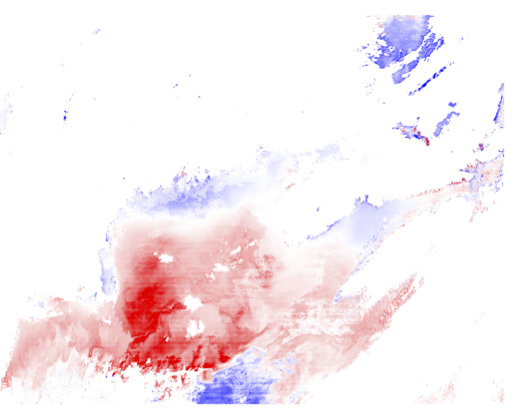
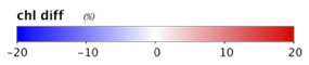
Revert to using the correct ancillary data for the remainder of this exercise.
9.2 Generate a Level-2 file with the vicarious gains all set to 1.0.
Rrs_443 differences from change in vicarious calibration:
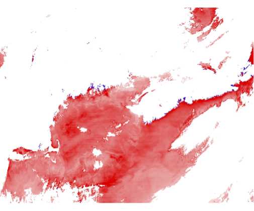

Revert to using the correct vicarious gains for the remainder of this exercise.
9.3 Generate a Level-2 file using SWIR bands instead of NIR bands in the atmospheric correction (set aer_wave_short=1240 and aer_wave_long=2130).
AOT_869 and angstrom differences from change in A/C bands:
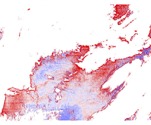
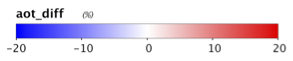
Revert to using the Level-2 files you created in Section 7 for the remainder of this lab.
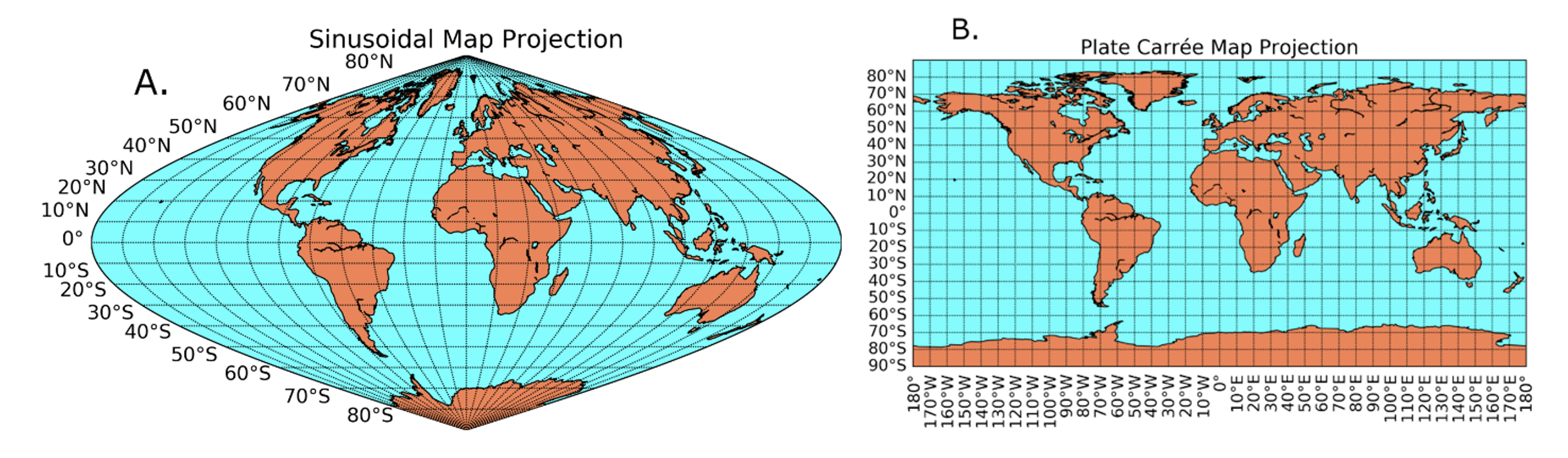
Someday, you may find yourself wanting or needing to re-grid (re-project) your Level-2 data onto a standard map grid. Here are examples of two common grids:
Note the differences in bin size as a function of latitude. Examine, e.g., Greenland.
One quick way to visualize the transformation from the satellite swath coordinate system to a standard map grid is to use OCSSW mapgen (formerly l2mapgen). This utility reprojects a Level-2 file onto a Plate Carree grid (panel B above) and generates a PNG or PNM image.
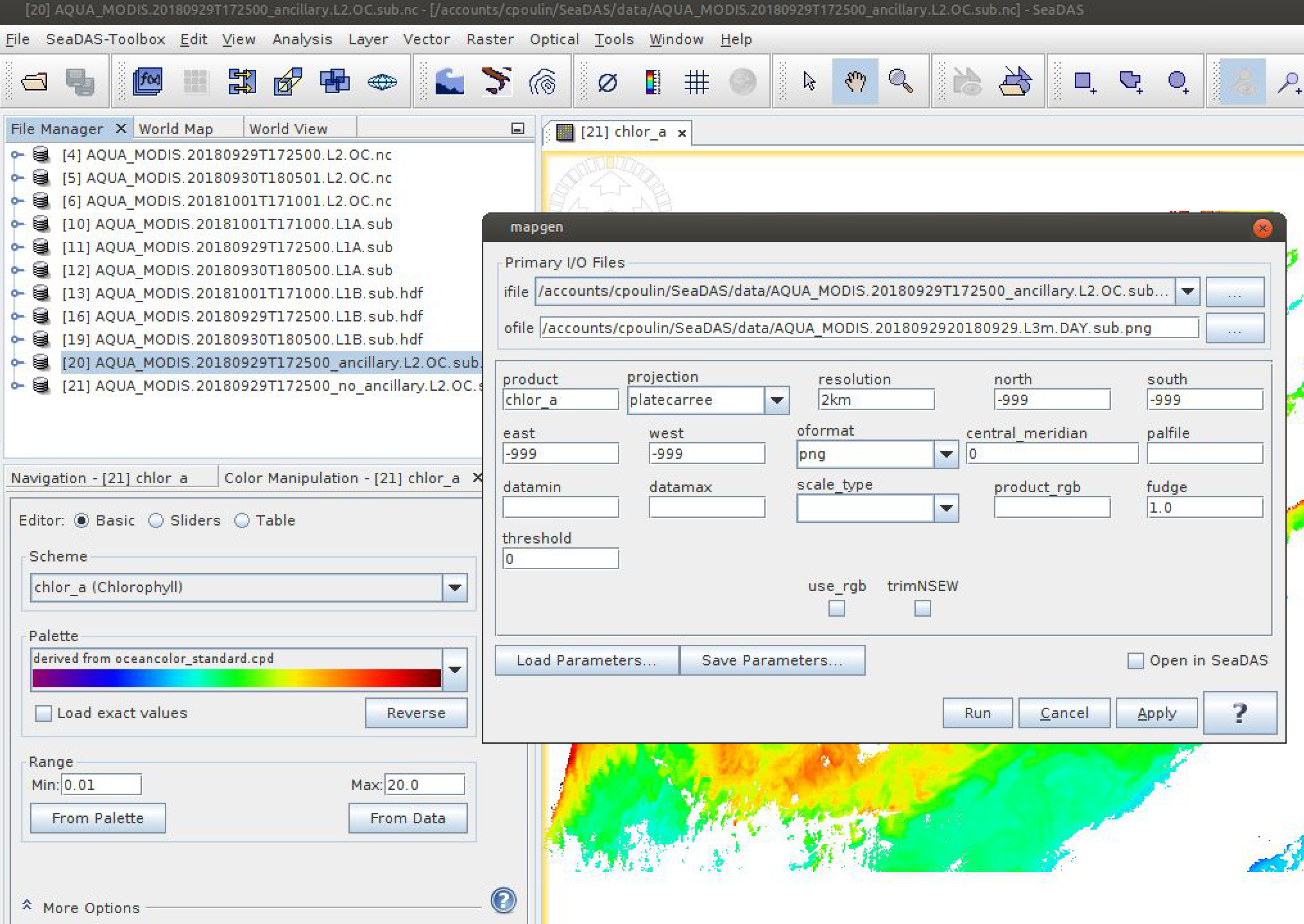
l2mapgen chlor_a:
The NASA processing cadence for producing Level-3 maps is:
(1) generate a Level-3 bin file, which is always in a sinusoidal map projection (panel A above) that retains equal distance in latitude and longitude space from north to south; then,
(2) generate the Level-3 map file in the projection of your choice (standard is Plate Carree). *SeaDAS cannot open Level-3 bin files.*
Let's next explore the effects of spatially re-gridding Level-2 data on geophysical values.
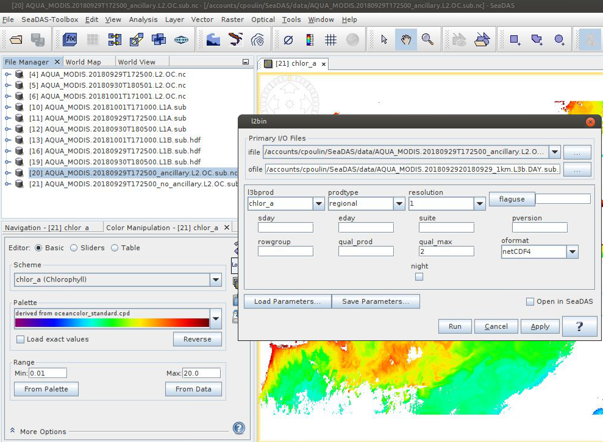
Use OCSSW l2bin to generate a series of chlor_a Level-3 bin files for
AQUA_MODIS.20180929T172500. Always set "l3bprod" to chlor_a. Always set
"prodtype" to regional. Run 4 times with "resolution" set to 1, 2, 4, and 9
km. Rename the ofile each time to avoid overwriting existing files.
Next, use OCSSW l3mapgen to convert these Level-3 bin files into Level-3 map files. Manually type "chlor_a" as the "product", leave the projection at "platecarree", and set the resolution to 1km, 2km, 4km, and 9km based on the resolution of the Level-3 bin file you are mapping.
This is a good time to revisit the help/usage information provided when running an OCSSW program without any input values . It's recommended that you do this for any program you plan to use to best understand the operation and options of that program.
Type
l3mapgen
in a terminal window.
Focus on usage for the "product" input. Note that you can modify an input product to report alternate statistics, such as standard deviations and the number of observations that filled each Level-3 grid-bin. Such information on capabilities is not always intuitive within a GUI environment. Best practices involve studying command line options.Open the original Level-2 and the 4 Level-3 mapped chlor_a products.
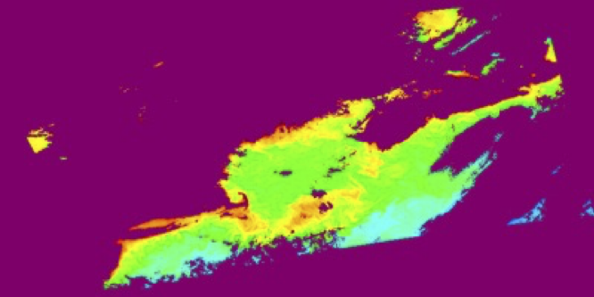
To explore how geophysical values change with re-gridding, let's focus on a
specific high chlorophyll area to the east of Cape Cod:
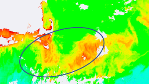
Quantify if/how this feature distorts relative to the Level-2 data when re-gridded at different spatial resolutions. You can do this through analysis of samples sizes, histograms or cumulative distributions, metrics of central tendency, or by other means of your choice. SeaDAS provides many options for such image analysis.
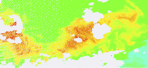
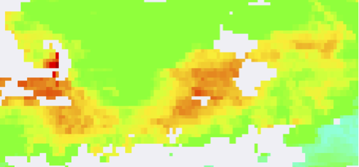
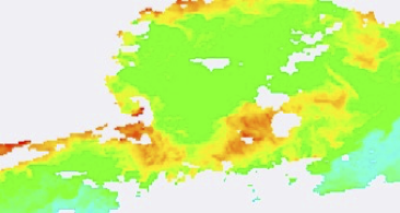
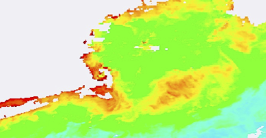
Level-2 vs. Level-3 maps at 1, 2, 4, and 9 km:
Level 2

Level 3, 1km
Level 3, 2km

Level 3, 4km
Level 3, 9km
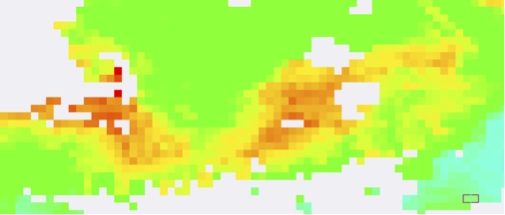
Now imagine that you're studying a small or filamentous feature, say a thin bloom of Trichodesmium offshore of Australia or Noctiluca in the Gulf of Oman.
The fine details of the bloom will be less apparent with a lower resolution.
Someday, you may find yourself wanting or needing to temporally composite your data into a longer term average (say, weekly, monthly or seasonally).
Use OCSSW l2bin to create regional 2-km chlor_a Level-3 bin files for the other two Level-2 files you generated in Section 7 (AQUA_MODIS.20180930T180500 and AQUA_MODIS.20181001T171000). When done, you should have 3 Level-3 2-km chlor_a bin files (one for each day).
We now want to create a single, temporal composite of these 3 files. We'll use OCSSW l3bin to do this, which will involve a different process than that for l2bin.
First, create a plain text file that lists the full name of all three Level-3 bin files to be composited, with one file name per line, for example:
A2018272.L3b_DAY_OC_2.sub

A2018273.L3b_DAY_OC_2.sub

A2018274.L3b_DAY_OC_2.sub
Select this text file as the ifile in the l3bin GUI. Next, type chlor_a as the prod and change the latitude and longitude boundaries to those we've been using in this lab (otherwise, you will create a global map … worth trying, though!).
After your 3-day Level-3 bin file has been created, use l3mapgen again to create a 2-km Level-3 map, as you did in Section 10.
1 day:
3-day:
?
Increased spatial coverage. Minimized impact of clouds in the scene.
?
Loss of geometry and temporal detail in the scene.
Small features risk being lost in temporal composites.
Level-2 images show more feature details than lower-resolution Level-3 images. Those details can be
useful to
identify phytoplankton communities.
Temporally composited level-3 images have a better spatial coverage than level-2 images, and help
reduce
the
effect of clouds on measurements. However, there is a loss of geometry and temporal detail in the
distribution
of phytoplankton.
Perhaps not widely known, OCSSW software within SeaDAS allows generation of geophysical data products from Level-3 Rrs bin files.
To explore this, we need to generate a Level-3 bin file that includes Rrs. Run l2bin on AQUA_MODIS.20180929T172500, but this time do not set assign a "l3bprod" in the GUI. Leaving this field blank will bin all products in the Level-2 file (if you ran l2bin from the command line without any inputs you should already know this). Do set prodtype to "regional" and resolution to "2".
*This is not currently working in SeaDAS 8.3*
Open the OCSSW l3gen GUI. Assign the Level-3 bin file you just created as ifile.
➜ Note that it looks and feels like the l2gen GUI, but without the ability to specify ancillary files. Why do you suppose this is?
Let's produce IOP products this time. Add adg_443_giop, aph_443_giop, and bbp_443_giop to the list of l2prods, either using the GUI buttons or by manually changing the field in the "Main" tab. Feel free to remove the rest of the l2prods. As always, rename ofile as necessary to avoid overwriting existing files.
Run l3gen. This will create a new Level-3 bin file with IOP products derived from Level-3 Rrs.
Run l3mapgen to convert this Level-3 bin file into a Level-3 map. Leaving the "product" field blank will create a map file containing all 3 IOP data products (again, you know this already if you ran l3mapgen from the command line to see its usage).
Level-3 data products do not contain information on geometry or time at the moment of measurement – all useful information for deriving some geophysical data products.
This is a good place to explore how different configurations of an IOP model influence the derived adg, aph, and bbp. Repeat this exercise, but use the "IOP Options" tab in the l3gen GUI to reparametrize GIOP.
End of laboratory. Nice work.